3. Understanding Transformer Architecture of LLM: Attention Is All You Need

What is RNN, LSTM:

Before to the Transformer models, some famous architectures we see in the field of natural language processing such as Recurrent Neural Networks (RNNs), Long Short-Term Memory (LSTM) networks, and Gated Recurrent Units (GRUs).

 

So what these models are for:

These architecture were particularly designed to handle sequential data and capture temporal dependencies effectively. These architecture are used in tasks for especially like language modeling and translation.While Recurrent Neural Networks (RNNs), including LSTM and GRUs, have been good in handling sequential data, they present several disadvantages compared to more modern architectures like Transformers:

• • Difficulty with Parallelization: As RNNs, LSTMs, and GRUs process data sequentially, each step depends on the previous one. And this significantly limits the possibility of parallelizing computations, so leading to longer training times, especially on large datasets.

• • Struggle with Long-range Dependencies: Despite improvements with LSTMs and GRUs, traditional RNNs often struggle to capture long-range dependencies within sequences. This is due to the vanishing gradient problem, where information from earlier steps becomes increasingly diluted as it passes through each timestep in long sequences.

• • Complexity and Efficiency: LSTMs and GRUs include mechanisms to mitigate issues like the vanishing gradient problem, but these additions make the architectures more complex and computationally intensive compared to simpler RNNs or even Transformers, which handle long sequences more efficiently through self-attention.

• • Scalability Issues: RNNs and their variants tend to be less scalable when dealing with extremely large datasets or models due to their sequential nature and slower training times, limiting their effectiveness for tasks that require analyzing vast amounts of data.

• • Difficulty in Learning Bidirectional Contexts; Resource Intensiveness

Despite these disadvantages, RNNs, LSTMs, and GRUs are still used in specific scenarios where model interpretability or understanding sequential data in its natural order is crucial. However, for many modern applications that require to handle of large datasets in less processing time, Transformers present a more efficient and effective solution so let’s talk about the transformer.

What is a Transformer?

A Transformer is a type of neural network architecture that has become fundamental in the field of deep learning, particularly for tasks involving natural language processing (NLP). Evolution from sequence models that process data linearly (RNNs, LSTMs) to models focusing on relevant parts of the data through attention mechanisms.It is a revolutionary shift or development in neural network. Transformer introduces self-attention mechanisms that enable the simultaneous or parallel processing of data points, meaning it efficiently uncovering complex hidden dependencies within the data. This parallel processing capability marks a significant evolution in the architecture of neural networks, enhancing their ability to handle large and complex datasets. Advantages of transformer in NLP: It Has significantly outperformed older models like RNNs and LSTMs on many NLP tasks due to its parallelization capabilities and efficiency.

Attention Is All You Need

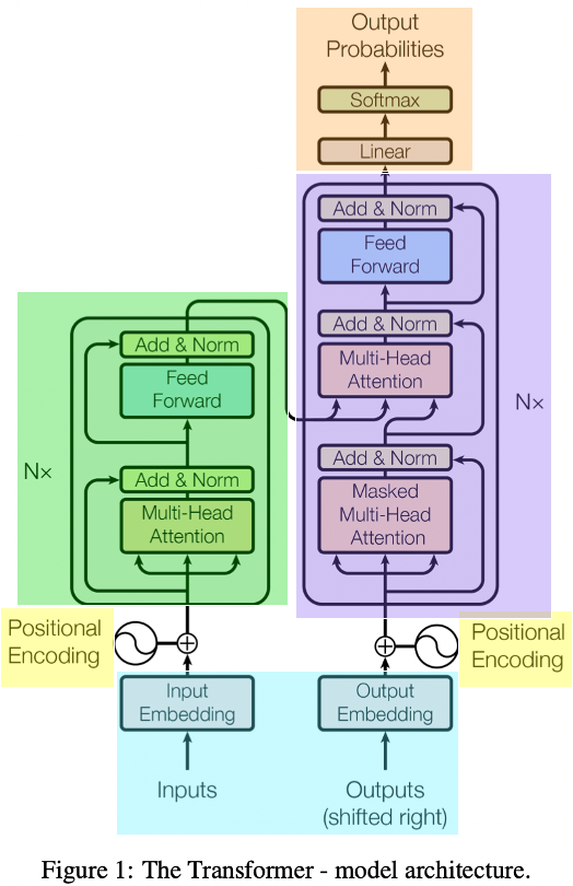
The Transformer model was first introduced in the paper “Attention Is All You Need” by Vaswani et al. in 2017. It revolutionized natural language processing by shifting away from recurrent layers to focus entirely on attention mechanisms. Originally designed for tasks such as translation and text comprehension, the architecture has since been adapted for diverse applications including image processing and music generation.

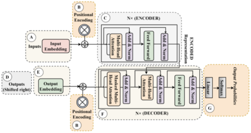
Transformer architecture

It is divided into two primary components: the encoder and the decoder.

• • Encoder: Each encoder layer works on the input sequence concurrently and includes two key sub-layers: a multi-head self-attention mechanism and a position-wise fully connected feed-forward network.

• • Decoder: Each decoder layer consists of three main sub-layers: a multi-head self-attention mechanism, a multi-head attention mechanism that attends to the encoder’s output, and a position-wise fully connected feed-forward network.

• • We can take example of a machine translation task: In which, the encoder processes the sentence in the source language, while the decoder incrementally generates the translation in the target language.

Input embedding layer

The inputs are the English words that we want to translate. The embedding layer maps each word into a high-dimensional space where similar words are closer to each other. It transform input tokens, such as words in text, into vectors of fixed size. let’s take an example sentence “sunset over the ocean”. In the context of a language model, each word in a sentence is converted into a vector. The embedding matrix contains a unique vector for each word in the vocabulary, effectively translating the textual information into numerical data that can be processed by the model.

 

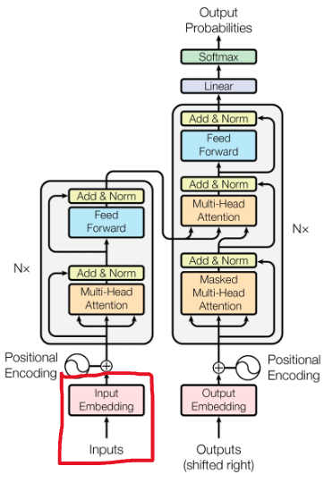
For instance, the word “Sunset” from our example sentence is turned into a numerical vector which might look something like [0.25, -0.75, 0.50, …, 0.10] within a high-dimensional space. This also captures various semantic and syntactic properties of the word within its dimensions. Likewise, the rest of the words  (“”, “over“, “the“, and “ocean“)  represents into a high-dimensional vector using an embedding matrix.

Positional encoding layer

It adds information about the position of each word in the sequence to the input embeddings, enabling the model to understand word order. Why positional encoding is important: We will continue with the same example that is sunset over the ocean. In here, sunset is the first word, and ocean word is at 4th place. Let’s swap the words these words and see the meaning that we were looking for. The meaning of the sentence is completely changed. That is the reason, transformer needs positional encoding. Next, we add a special marker to each word that shows its position in the sentence. So We added positional encodings to each word embedding matrix to convey their positions in the sequence. So, for “sunset, we add something like [0.25, -0.75, 0.50, …, 0.10, 1] to indicate it’s the first word. For “over”, it might become [0.1, -0.7, 0.6, …, -0.4, 2], showing it’s the second word, and so on. This helps the model understand the order of words in the sentence.

 

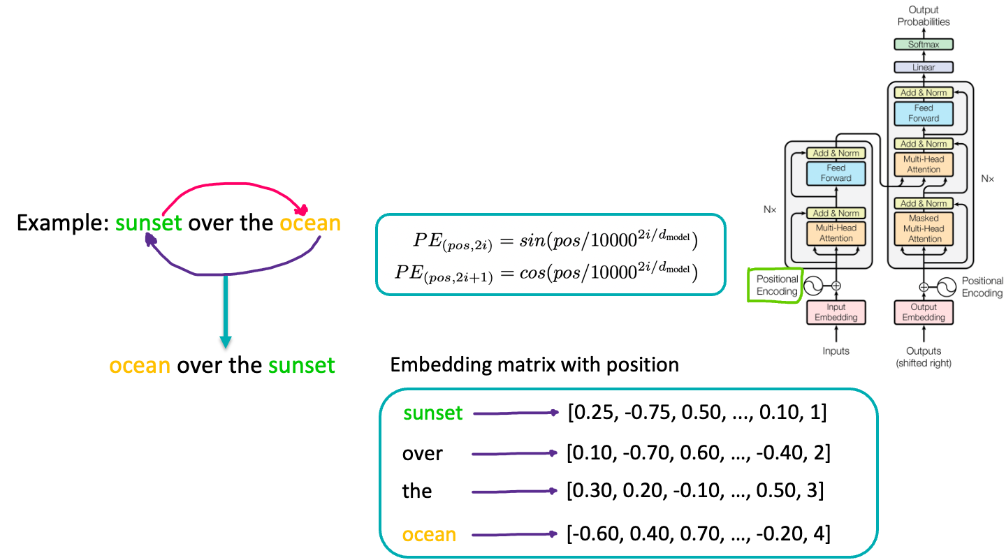
In summary, positional encoding adjusts the embedding vector to accurately represent token position within the sequence. The architecture add “positional encodings” to the input embeddings at the bottoms of the encoder and decoder stacks. 

Formula:

• • PE stands for “Positional Encoding”.

• • pos refers to the position of the word in the sentence.

• • i is the dimension index of the positional encoding.

• • d_model is the dimensionality of the model’s input word embedding, typically in the range of 512 or 768, etc.

• • The term 10000²ⁱ/d_model is a scaling factor that causes the sine and cosine functions to have wavelengths that form a geometric progression from 2π to 10000⋅2𝜋. This allows the model to easily learn to attend by relative positions since for any fixed offset k, PE_(pos+k) can be represented as a linear function of PE_(pos).

• • The even indices (2i) use the sine function and the odd indices (2i+1) use the cosine function. This pair of equations generates a unique positional encoding for each position and for each dimension of the word embedding, which then gets added to the embedding itself.

• • The use of sine and cosine is purposeful as they are functions that can be easily summed and have values between -1 and 1, so they are bound and can be directly added to the scaled embedding vectors without disrupting the original information too much. Moreover, because these functions are periodic, they allow the model to generalize to sequence lengths longer than the ones encountered during training.

Encoder Layer

It processes the input sentence. It has multiple identical layers (Nx). Each layer has two sub-layers. The first sub-layer is the multi-head self-attention mechanism. The second is a position-wise fully connected feed-forward network

 

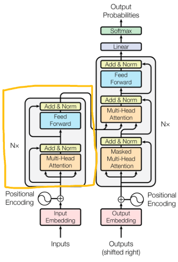
Multi-Head Attention (within Encoder) layer

Multi-Head Attention is an important component within the Transformer architecture, particularly within the encoder. Imagine the model has several monitor, each focusing on different parts of the sentence at the same time. Each monitor (or we can call head) looks at the words and decides how important they are to each other. So, for “sunset over the ocean“, one monitor might focus on “sunset” and “ocean” while another monitor focuses on “over” and “the” words. Meaning, they calculate how much attention each word should give to the others based on their meanings and positions. For instance, The model might focus on “sunset” and “ocean” simultaneously because they are related, creating a contextual representation of “sunset” that includes its relationship with “ocean.”

 

Let’s get into some mathematical foundation:

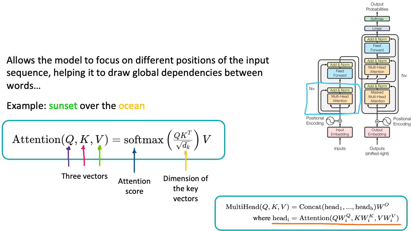
Attention Equation:

Attention(Q, K, V) = softmax((QK^T) / sqrt(d_k)) V: This is the formula for calculating attention weights. It computes how much attention to pay to each word when considering another word.

• • Q, K, V: These represent the “query,” “key,” and “value” vectors respectively. Each word in the sentence is mapped to these three vectors. In our context, “Q” might be related to the word “sunset,” while “K” and “V” are associated with “over” and “ocean.”

• • Attention Score: This score is calculated by taking the dot product of the “query” with all “keys” (QK^T), indicating the relevance of other words’ “keys” to the current “query.”

• • Dimension of the key vectors: dk is the dimensionality of the key vectors. The square root of dk is used to scale the attention scores, which helps in stabilizing gradients during training.

• • Softmax Function: Applied to turn the scores into probabilities, indicating the amount of attention one word should give to others.

• • V (Values): Once the attention probabilities are calculated, they’re used to create a weighted sum of the “value” vectors, which becomes the output of the attention step.

Multi-Head Attention Formula:

MultiHead(Q, K, V) = Concat(head1, …, headh) W^O: This shows how the individual attention outputs from multiple ‘heads’ are combined into a single output.

• • head = Attention(QW_i^Q, KW_i^K, VW_i^V): In highlighted part, each head applies attention to different projected versions of the queries, keys, and values. This is like having multiple ‘perspectives’ on the input sentence, each focusing on different relationships between the words.

• • Concatenation: The outputs from each head are concatenated.

• • W^O: A weight matrix that combines the concatenated outputs into a single vector that retains information from all the heads.

To sum up, in the multi-lead attention layer, the explained process happens multiple times in parallel (or multiple ‘heads’), allowing the model to capture different types of relationships between words (e.g., syntactic and semantic).

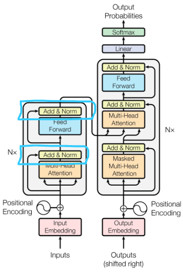
Add & Norm layer

Each attention output is then added to the original input vector (residual connection) to preserve the information through the layers of the network. Afterward, normalization is applied to stabilize the learning process. After attention processing, each vector is normalized to stabilize learning and integration, ensuring smooth and efficient training of the model.

 

Point-wise Feed Forward networks layer

In the context of the transformer architecture, the position-wise feed-forward networks (FFN) are another key component alongside the attention mechanisms. The Transformer uses these feed-forward networks in both the encoder and decoder, and they operate on each position separately but in the same way. This means that for each position in the sequence — say, for each word in our sentence — the same feed-forward network is applied. But, it’s important to note that even though the process is the same, each position has its own inputs and thus its own outputs.

 

The feed-forward network consists of two linear transformations with a ReLU activation in the middle. 

1. 1. First Linear Transformation: takes input “sunset”  and multiplies by a weight matrix W1,  and then adds a bias term b1 into it. This is the first transformation, which changes the representation of “sunset” into a different space, possibly with a higher dimension.
   2. ReLU Activation: afterwords, the transformed version of “sunset” is then passed through a ReLU (Rectified Linear Unit) activation function. The ReLU function keeps any positive values as they are and changes any negative values to zero.
   3. Second Linear Transformation: After ReLU has done its job, the result goes through second linear transformation with a new weight matrix 𝑊2 and bias term 𝑏2. This second transformation typically maps the representation back to the original dimension of the model.

The position-wise feed-forward networks allow the Transformer to learn even more about the relationship between words in the sentence because they can modify the output of the attention layers at each position 

Decoder

The decoder also consists of layers that mainly focus on generating the translated output step-by-step. The decoder is generating the translated sentence in Spanish one word at a time. It has a similar structure to the encoder, but with the addition of a third sub-layer that performs multi-head attention over the encoder’s output. Each layer in the decoder uses both self-attention to look at previous words in the output and encoder-decoder attention to focus on relevant parts of the input sentence.

 

For example: As the decoder starts generating the translation “Puesta de sol sobre el océano”, it uses the refined outputs from the encoder to select which Spanish words to generate based on the context provided by “Sunset over the ocean”. The encoder-decoder attention helps focus on “Sunset” when deciding how to translate it into “Puesta de sol”.

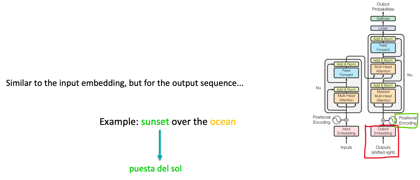
Output embedding and position encoding layers

Taking about output embedding and position encoding, it is similar to the input embedding, but for the output sequence. Translates each predicted word into a vector and adds positional information.  As the model begins to translate our sentence, the word “puesta del sol” (for “Sunset”) would get its own embedding and positional encoding.

• • Masked Multi-Head Attention: In the decoder, multi-head attention needs to be masked to prevent the model from seeing the future tokens it has yet to predict. This ensures that the predictions are autoregressive.

• • Add & Norm and Feed Forward: These are similar to the encoder’s layers but are specific to the decoder’s architecture.

 

Linear and softmax layers

Finally, The linear layer maps the decoder’s output to a much larger vector, with the size usually equal to the vocabulary. A softmax layer then converts these scores to probabilities, and the word with the highest probability is chosen as the translation. The process continues until an end-of-sequence token is generated.

 

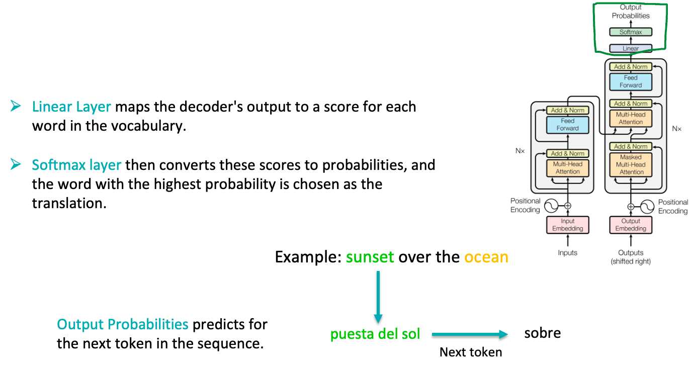
Output Probabilities: These are the final probabilities for each word in the target language vocabulary that the model predicts for the next token in the sequence.For example, The word “puesta del sol” gets transformed into a probability distribution over all possible next words, and softmax determines that “sobre” is the most likely next word in the translation.

Applications

Transformer models are not just theoretical; they’re applied in machine translation, text summarization, and even in identifying names and places in texts—showcasing their versatility and power.

That is all for this post! See you in next! 🙂

Happy reading:)