1. KAN: Kolmogorov–Arnold Networks Method

Before we enter into the paper details we see the title and author of the paper.

Research paper about “Kolmogorov-Arnold Networks” (KAN), a topic related to a specific type of neural network or mathematical model. The authors of the paper from the institutions such as MIT, Caltech, and Northeastern University. This is a recent and possibly cutting-edge study in the field of artificial intelligence or computational mathematics.

In this paper we see methods comparison mainly with the Multi-layer Perceptrons (MLPs) so I thought of including a basics things about MLP.

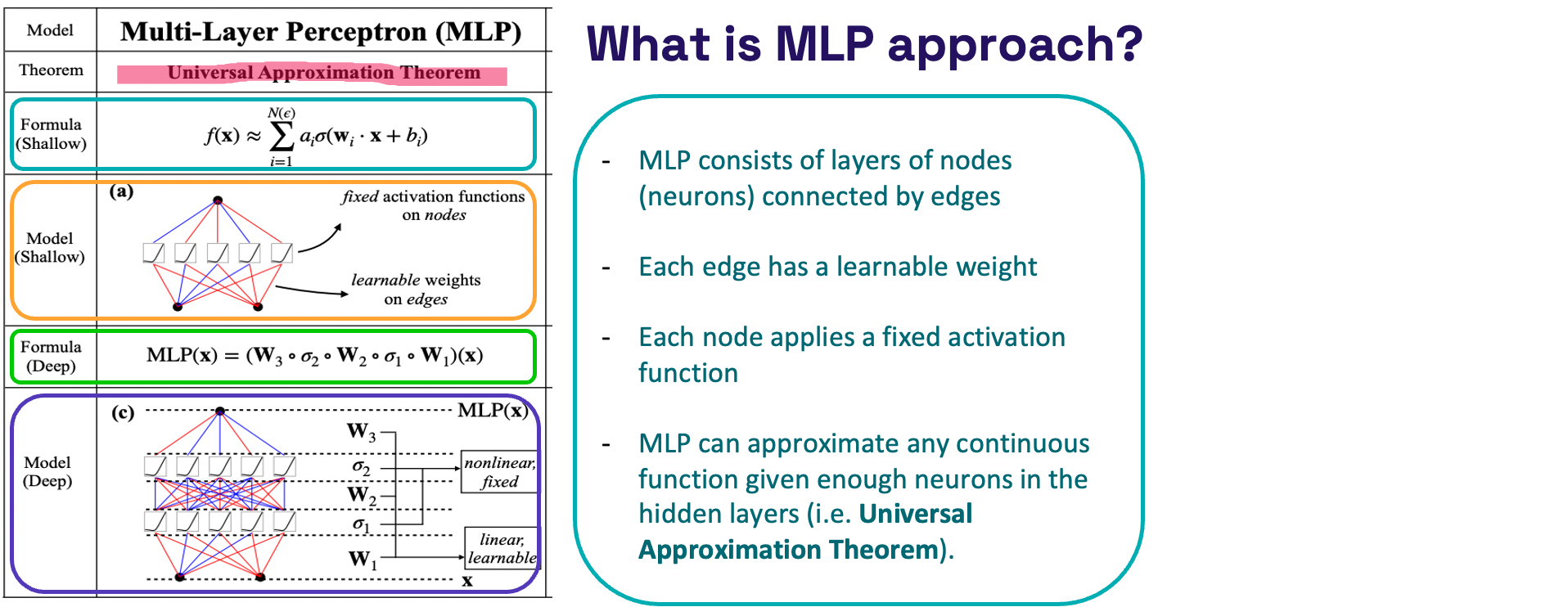
What is MLP approach?

1. Model – The Figure below shows a basic representation of an MLP, which consists of layers of nodes (neurons) connected by edges. Each edge has a learnable weight, and each node applies a fixed activation function.
2. Universal Approximation Theorem – This theorem is highlighted, stating that MLPs can approximate any continuous function given enough neurons in the hidden layers.
3. Formulas – Two formulas are presented:

   • Shallow Formula: Represents a single hidden layer MLP where f(x) ≈ ∑(w_i * x + b_i) with σ as the activation function.
   • Deep Formula: Shows the composition of multiple layers in an MLP: MLP(x) = (W₃∘σ₂∘W₂∘σ₁∘W₁)(x), illustrating how inputs x are transformed through layers by alternating linear transformations (W matrices) and fixed nonlinear activations (σ).

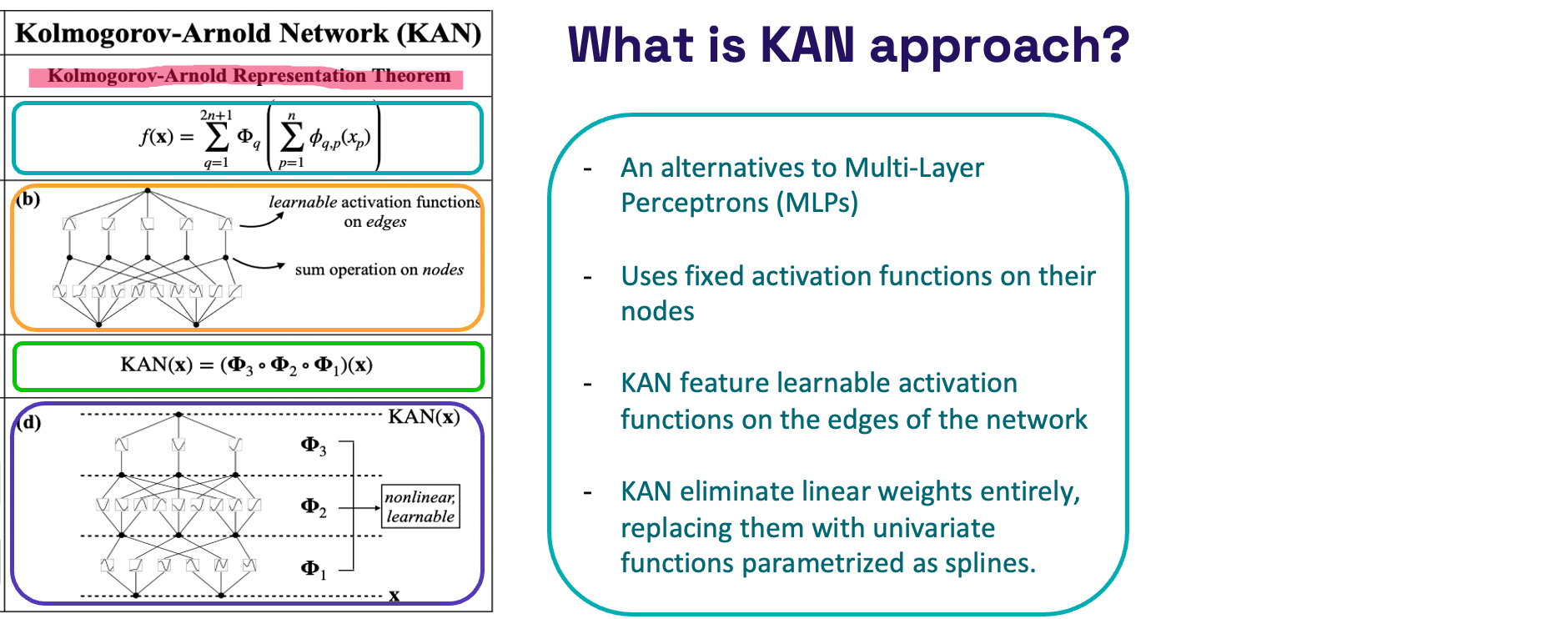
What is KAN approach?

Now we will see what is novel approach published two weeks before, which is aim of this post:

1. Kolmogorov-Arnold Representation Theorem:

   • States that any continuous function can be represented through a combination of simpler, continuous functions.
   • The formula provided, shows how a complex function can be decomposed into a series of operations involving simpler functions.

2. Structure of the Network:

   • Diagram (b): Displays the structure of KAN, where each edge has a learnable activation function and each node performs a summation of its inputs.
   • Diagram (d): Breaks down the network into three layers (Φ₁,Φ₂,Φ₃), where each layer processes the outputs of the previous layer through nonlinear, learnable functions.

3. KAN(x) Equation:

   • 𝐾𝐴𝑁(𝑥)=(Φ₃∘Φ₂∘Φ₁)(x) describes how an input 𝑥 is transformed sequentially by three layers, with each layer applying a specific transformation and passing the result to the next.

4. KAN Approach:

   • KAN is proposed as an alternative to traditional multi-layer perceptrons, which typically use fixed activation functions.
   • Learnable Activation Functions: Unlike MLPs, KANs incorporate activation functions on the edges that are adaptable, allowing the network to learn more flexible representations.
   • Elimination of Linear Weights: KANs do not use linear weights. Instead, they use univariate functions parameterized as splines to model relationships, offering potentially greater flexibility and control over the model’s behavior.

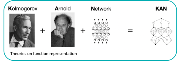
Authors: Kolmogorov–Arnold Networks

Scientist, Andrey Kolmogorov contributed foundational theories in the function space, mainly a representation theorem that tells any multivariate continuous function can be represented as a superposition of continuous functions of one variable.

Scientist, Vladimir Arnold extended Kolmogorov’s work, contributed further to understand of these function approximations, mainly in how these functions interact in complex systems.

When you combine their theoretical contributions with the architecture of a neural network, which mainly involves nodes (neurons) connected by edges  that can process and transmit information via mathematical functions, and you get the KAN model.

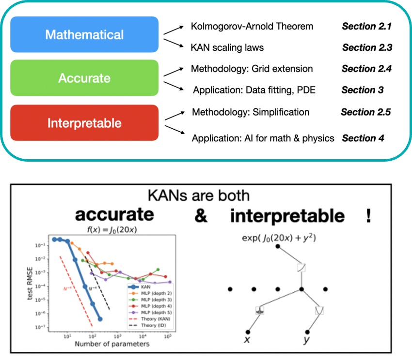
Mathematical, Accurate, Interpretable

In here, the paper highlights mathematical basis, accuracy, and interpretability as key strengths of KANs. Also, the study compared KANs with traditional multi-layer perceptrons. KAN shows good performance and efficiency in parameter use. Also, KANs are not just theoretically robust but also highly effective in practical applications.

B-spline activation function

The Figure 2.2 shows a neural network where B-spline functions are used as activation functions. The right side of the figure shows how a single B-spline activation function, represented as 𝜙(𝑥), is composed of a weighted sum of basis splines, 𝐵_𝑖(𝑥). The coefficients, 𝑐𝑖 determine the shape of the B-spline, which can be adjusted to adapt to more detailed data representations by increasing the number of knots and basis functions. This adaptability allows for more precise modeling in the neural network.

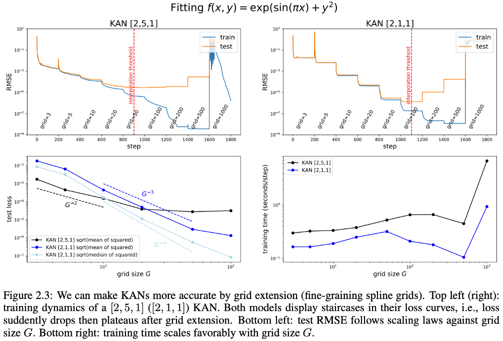
Fine-graining spline grids

The Figure 2.3 shows how increasing the grid size in KAN improves their ability to accurately model a complex mathematical function. Additionally, the graphs show a pattern of sharp drops in error when the grid size is increased.

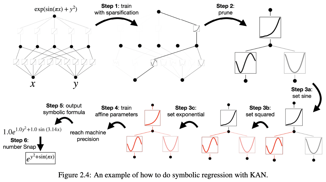
Symbolic regression with KAN

The Figure 2.4 outlines a systematic process of symbolic regression using a Kolmogorov-Arnold Network (KAN), detailing how to efficiently derive symbolic formulas from data. Here are the key steps:

1. Train with Sparsification:

   • The network starts by training on the data while applying sparsification techniques to ensure the model focuses on the most relevant features, reducing complexity and enhancing interpretability.

2. Prune:

   • After initial training, the model is pruned, which involves removing less significant connections or nodes, simplifying the network further without losing critical information.

3. Set Specific Functions:

   • Step 3a: Nodes are set to represent specific functions such as sine.
   • Step 3b: Other nodes may be set to represent other mathematical operations, such as squaring the input.
   • Step 3c: Additional nodes might be configured to represent exponential functions, completing the set of basic mathematical constructs used in the model.

4. Train Affine Parameters:

   • Further training is done to fine-tune the affine parameters (constants and coefficients) within the symbolic expressions identified in the previous steps.

5. Output Symbolic Formula:

   • The network then outputs a symbolic formula, providing a mathematical representation of the data relationships it has learned.

6. Number Snap:

   • Finally, a ‘number snap’ is applied to the output formula to adjust numerical values to more standardized or meaningful figures, further refining the model’s accuracy and interpretability.

This process effectively translates complex data into a concise, symbolic mathematical expression through a series of steps that simplify, prune, and specify the network’s structure and function, leading to an optimized and interpretable model.

KAN and MLP comparison

The Figure 3.1 provides a comparative analysis between Kolmogorov-Arnold Networks (KANs) and Multi-Layer Perceptrons (MLPs) across five different mathematical functions, focusing on how the number of parameters affects the test Root Mean Square Error (RMSE). 

Here are some key points highlighted in the graphs:

1. Function Types:

   • The comparison involves several types of functions, including Bessel functions (𝐽₀(20𝑥)), exponential and trigonometric combinations (exp⁡(sin⁡(𝜋𝑥)+𝑦²)), products (𝑥𝑦), complex summations (exp⁡(∑𝑖=1100sin⁡2(𝜋𝑥𝑖2)), and multi-variable exponential trigonometric functions (exp⁡(sin⁡(𝑥1²+𝑦2²)+sin⁡(𝑥3²+𝑧4²)).

2. Depth Variations:

   • Both KANs and MLPs are analyzed at various depths (2 to 5), allowing for a comparison of performance relative to network complexity.

3. Performance Metrics:

   • The test RMSE is plotted against the number of parameters in a logarithmic scale. Lower RMSE values indicate better model accuracy.

4. Comparison Results:

   • KANs generally show a steeper decline in RMSE with fewer parameters compared to MLPs, suggesting that KANs require fewer parameters to achieve similar or better accuracy.
   • MLPs show a trend of slow improvement and quick varying in RMSE as the number of parameters increases, indicating diminishing returns on model complexity.

5. Theoretical Predictions:

   • The dashed lines represent theoretical predictions for KANs and a one-dimensional (ID) theory, showing that KANs align closely with the theoretical model, particularly in scenarios involving fewer parameters.

This comparison underscores KANs’ efficiency and effectiveness in handling complex functions with fewer parameters compared to traditional MLP architectures, highlighting their potential for more scalable and efficient modeling in various applications.

Fitting special functions

The Figure 3.2 presents a comparative analysis between Kolmogorov-Arnold Networks (KANs) and Multi-Layer Perceptrons (MLPs) in terms of fitting various specialized mathematical functions, with performance measured by the Root Mean Square Error (RMSE) and the number of parameters used. Here are the key points:

1. Special Functions Tested: The functions include elliptic integrals (ellipj, ellipkinc, ellipeinc), modified Bessel functions (kv, iv), spherical harmonics (sph_harm_m_0_n_1 and others), and Bessel functions of the first kind (jv, yv).
2. Performance Metrics: Each chart plots RMSE against the number of parameters, comparing the performance of KANs and MLPs in both training and testing phases.
3. KAN Performance: In almost all cases, KANs show a more favorable decrease in RMSE with an increase in the number of parameters, indicating they require fewer parameters to achieve lower error rates compared to MLPs.
4. MLP Performance: MLPs generally exhibit higher RMSEs at similar parameter counts, and their curves tend to plateau sooner, indicating diminishing returns on accuracy with additional parameters.
5. Pareto Frontier Comparison: The analysis suggests that KANs consistently position closer to the Pareto frontier in these tests, demonstrating that they provide a better trade-off between the number of parameters and the accuracy of fitting these specialized functions.
   

This comparison highlights KANs’ effectiveness and efficiency in modeling complex functions with fewer parameters compared to traditional MLPs, offering potential advantages in applications requiring precise mathematical modeling with efficient parameter usage.

Continual Learning Problem

The provided Figure 3.3 demonstrates the advantages of Kolmogorov-Arnold Networks (KANs) over Multi-Layer Perceptrons (MLPs) in a continual learning problem involving a 1D regression task with Gaussian peaks. Here are the key points from the Figure:

1. Learning Dynamics:

   • The first two graphs compare the L2 and H1 squared losses (measuring error in solutions) for KANs and MLPs over training steps. KANs show faster convergence and lower losses compared to MLPs, indicating a quicker and more efficient learning process.

2. Scaling of Losses:

   • The third and fourth graphs depict the scaling of L2 and H1 losses against the number of parameters. KANs demonstrate steeper and more favorable scaling laws, suggesting that they achieve lower losses with fewer parameters, enhancing model efficiency.

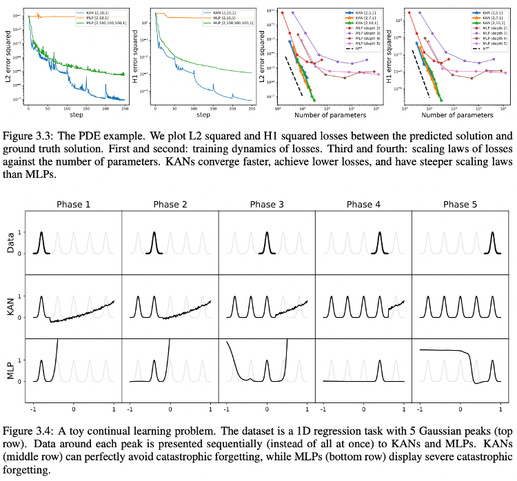
Let’s discuss the Figure 3.4,

1. Continual Learning Performance:

   • In here, a toy continual learning scenario is presented, where the model sequentially learns data around each of five Gaussian peaks. 
   • The top row shows the original data for each phase.

2. Model Comparisons in Continual Learning:

   • The KAN row (middle) and the MLP row (bottom) show each network’s learning outcomes across five phases. 
   • KANs adapt to new data without forgetting previous patterns, indicating effective continual learning and memory retention. 
   • In contrast, MLPs exhibit catastrophic forgetting, where they fail to retain earlier learned patterns as new data is introduced.

3. Effectiveness of KANs in Complex Learning Scenarios:

   • The overall results emphasize KANs’ superior capability in handling complex learning scenarios like continual learning, where maintaining past knowledge and integrating new information efficiently is crucial.

This effectively shows how KANs are potentially more suitable for tasks requiring robust continual learning and adaptation compared to traditional MLPs.

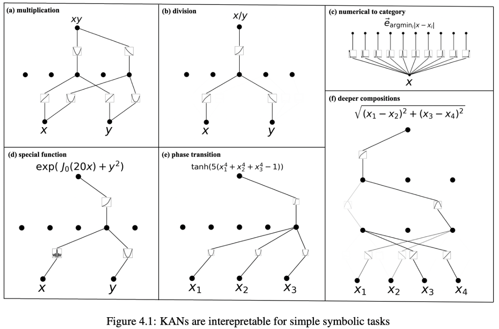
Interpretable

The Figure 4.1 illustrates the interpretability of Kolmogorov-Arnold Networks (KANs) in representing various symbolic mathematical operations and tasks.

Here are the key points depicted through different panels in the figure:

1. Multiplication (Panel a):

   • Shows a KAN structure for computing the product of two inputs, 𝑥 and 𝑦. The network combines these inputs to produce the output 𝑥𝑦, showcasing KAN’s capability to perform basic arithmetic operations.

2. Division (Panel b):

   • Depicts a KAN configuration for division, where x is divided by 𝑦 to yield x/y. This illustrates the adaptability of KANs to handle fundamental arithmetic operations.

3. Numerical to Category (Panel c):

   • Displays a more complex KAN setup for converting numerical input X into a categorical output. This demonstrates KAN’s use in tasks requiring classification based on numerical closeness, using operations like the argmin function.

4. Special Function (Panel d):

   • Represents a KAN structure for evaluating a special mathematical function, exp⁡(𝐽0(20𝑥)+𝑦²), highlighting KAN’s ability to integrate complex mathematical functions and exponential operations.

5. Phase Transition (Panel e):

   • Illustrates a KAN model computing a tanh function of a polynomial expression, indicative of KAN’s potential in complex transformations and activations used in neural network layers.

6. Deeper Compositions (Panel f):

   • Shows a more intricate KAN setup that calculates the Euclidean distance between points (𝑥₁,𝑥₂) and (𝑥₃,𝑥₄), further showcasing the network’s ability to handle geometric and spatial computations.

These panels collectively highlight how KANs are not only capable of handling basic and complex mathematical operations but also demonstrate their versatility and interpretability in various computational tasks, making them a powerful tool in symbolic regression and other advanced mathematical modeling.

Unsupervised Learning

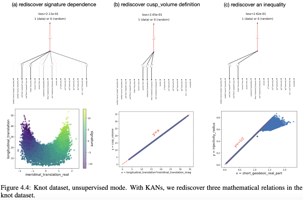
The Figure 4.4 illustrates the application of Kolmogorov-Arnold Networks (KANs) to rediscover mathematical relationships within the Knot dataset. 

Here are the key points from the Figure:

1. Panel (a) – Rediscover Signature Dependence:

   • Shows how KANs can identify dependencies within the dataset by using all available variables. The scatter plot below the network structure visualizes the relationship between ‘meridinal_translation_real’ and ‘longitudinal_translation’, with color indicating ‘faith’, highlighting how these variables are interrelated.

2. Panel (b) – Rediscover Cusp Volume Definition:

   • Demonstrates KANs’ capability to identify a precise mathematical relationship, specifically a cusp volume definition shown by the formula 𝑦=𝑥 in the scatter plot. This plot aligns data points along the line 𝑦=𝑥, verifying the network’s ability to capture linear relationships accurately.

3. Panel (c) – Rediscover an Inequality:

   • Illustrates KANs’ effectiveness in discovering inequalities within the data. The scatter plot shows a clear linear trend represented by the inequality 𝑦≤𝑥+1/2, where the data points predominantly fall below or on the line, emphasizing the network’s capacity to delineate boundaries and constraints within dataset features.

These panels collectively demonstrate the robustness of KANs in unsupervised learning to extract and visualize fundamental mathematical relationships and constraints from complex datasets without prior labeling or explicit guidance. This ability makes KANs particularly valuable for exploratory data analysis and in situations where underlying data structures are unknown or need to be clarified.

Should I use KAN or MLP?

The section presents a decision-making framework to determine whether to use Kolmogorov-Arnold Networks (KANs) or Multi-Layer Perceptrons (MLPs) based on various criteria related to accuracy, interpretability, and efficiency (see the Figure below). Here are the highlighted decision points:

1. Accuracy:

   • Compositional Structure: If your problem requires modeling compositional structures, choose KANs.
   • Complicated Function: For problems involving complicated functions, KANs are preferable.
   • Continual Learning: KANs are recommended if your task involves continual learning, where the ability to learn continually without forgetting is crucial.

2. Interpretability:

   • Dimension: If dealing with high-dimensional data, KANs are advisable because they might offer clearer insights due to their compositional nature.
   • Level: For tasks where interpretability is a priority, particularly at a qualitative level, KANs are generally preferred due to their transparent structure.

3. Efficiency:

   • Want Small Models: If the goal is to minimize model size, KANs are recommended as they can be more parameter-efficient.
   • Want Fast Training: For scenarios where fast training is crucial, MLPs might be the better choice as they are typically less complex to train compared to KANs which might require more intricate setups for training.

This framework helps in selecting the appropriate network type based on specific needs and constraints of the task at hand, focusing on the strengths of each type of network in handling different aspects of machine learning tasks.

That is all for this post! See you in the next post!

Happy reading!:)